Overview
Part 1 looks at some principles and introduces some of the tools in your arsenal.
Part 2 covers the dreaded PostgreSQL bloat issue as well as how TOAST can help performance, or hinder it.
Part 3 (this post) dives deeper into identifying, investigating and mitigating slow queries.
Part 4 covers indexing.
Part 5 covers rewriting queries.
TL;DR
- Use logging to identify slow queries
- Use
EXPLAINto examine an explain plan EXPLAIN (ANALYZE)can be dangerous!- Use depesz, dalibo or PEV to visualize your explain plan
- Red flags in your explain plan include filters, Rows Removed, and / or costs in excess of 100,000
- Data may not be evenly distributed, check it! Especially test data!
- Only select the rows and columns you need
Identifying slow queries
The most reliable way of identifying slow queries is to enable slow query logging using the parameter log_min_duration_statement. The pain threshold varies by environment, but for example if you wanted to log all queries that take longer than 50ms, you would issue the following command in psql:
set log_min_duration_statement=50;
You can also set this as a configuration parameter.
This results in messages in the PostgreSQL logs like:
...
2023-03-11 17:20:27.262 UTC [119] LOG:  duration: 54.77 ms  statement: insert into abc values(1);
2023-03-11 17:20:29.281 UTC [119] LOG:  duration: 86.56 ms  statement: insert into abc values(2);
2023-03-11 17:20:34.151 UTC [119] LOG:  duration: 72.63 ms  statement: insert into abc values(3);
2023-03-11 17:20:40.473 UTC [119] LOG:  duration: 336.449 ms  statement: select count(1) from abc;
...
EXPLAIN
The EXPLAIN command is used to show you have PostgreSQL is approaching the query. It has several useful variants which can be used together to give you a comprehensive overview of the query plan in human readable(-ish!) form. Each block of the resulting plan is called a node.
ANALYZE- Execute the query to return actual times
BUFFERS- Show buffer usage details (requires ANALYZE)
COSTS- Show estimated startup and total cost of each node
SETTINGS- Show non-default settings that affect the query plan
VERBOSE- Adds useful information to a plan
FORMAT JSON- The FORMAT can be TEXT, XML, JSON, or YAML. TEXT is the default and is human-readable. JSON is used by most of the explain plan visualizers we will be discussing shortly.
A first-cut EXPLAIN might be:
EXPLAIN (COSTS, SETTINGS, VERBOSE) SELECT count(1) FROM abc;
If you’re certain that executing the statement is not a problem, you might progress to;
EXPLAIN (ANALYZE, BUFFERS, COSTS, SETTINGS, VERBOSE) SELECT count(1) FROM abc;
If you then want to submit the explain plan to a visualization tool, such as pev, you would opt for:
\a
\t
\pset pager off
EXPLAIN (ANALYZE, BUFFERS, COSTS, SETTINGS, VERBOSE, FORMAT JSON) SELECT count(1) FROM abc;
As an example, I’ve used pgbench with 100 branches and the following row counts:
bench=# select count(*) from pgbench_accounts pa join pgbench_history ph on pa.aid = ph.aid where pa.bid != ph.bid;
 count
--------
 442066
(1 row)

bench=# select count(*) from pgbench_accounts pa join pgbench_history ph on pa.aid = ph.aid where pa.bid = ph.bid;
 count
-------
  4390
(1 row)

bench=# select count(*) from pgbench_accounts pa join pgbench_history ph on pa.aid = ph.aid;
 count
--------
 446456
(1 row)
A non-ANALYZE explain:
bench=# explain (costs, settings, verbose) select count(*) from pgbench_accounts pa join pgbench_history ph on pa.aid = ph.aid where pa.bid != ph.bid;
                                                       QUERY PLAN
------------------------------------------------------------------------------------------------------------------------
 Finalize Aggregate  (cost=237837.61..237837.62 rows=1 width=8)
   Output: count(*)
   ->  Gather  (cost=237837.40..237837.61 rows=2 width=8)
         Output: (PARTIAL count(*))
         Workers Planned: 2
         ->  Partial Aggregate  (cost=236837.40..236837.41 rows=1 width=8)
               Output: PARTIAL count(*)
               ->  Parallel Hash Join  (cost=8760.97..236376.99 rows=184162 width=0)
                     Hash Cond: (pa.aid = ph.aid)
                     Join Filter: (pa.bid <> ph.bid)
                     ->  Parallel Seq Scan on public.pgbench_accounts pa  (cost=0.00..210602.60 rows=4172160 width=8)
                           Output: pa.aid, pa.bid, pa.abalance, pa.filler
                     ->  Parallel Hash  (cost=5478.21..5478.21 rows=262621 width=8)
                           Output: ph.aid, ph.bid
                           ->  Parallel Seq Scan on public.pgbench_history ph  (cost=0.00..5478.21 rows=262621 width=8)
                                 Output: ph.aid, ph.bid
(16 rows)

Time: 2.435 ms
Now with ANALYZE:
bench=# explain (analyze, buffers, costs, settings, verbose) select count(*) from pgbench_accounts pa join pgbench_history ph on pa.aid = ph.aid where pa.bid != ph.bid;
                                                                               QUERY PLAN
-------------------------------------------------------------------------------------------------------------------------------------------------------------------------
 Finalize Aggregate  (cost=237837.61..237837.62 rows=1 width=8) (actual time=3942.519..3945.996 rows=1 loops=1)
   Output: count(*)
   Buffers: shared hit=16281 read=155614
   ->  Gather  (cost=237837.40..237837.61 rows=2 width=8) (actual time=3941.358..3945.984 rows=3 loops=1)
         Output: (PARTIAL count(*))
         Workers Planned: 2
         Workers Launched: 2
         Buffers: shared hit=16281 read=155614
         ->  Partial Aggregate  (cost=236837.40..236837.41 rows=1 width=8) (actual time=3903.302..3903.304 rows=1 loops=3)
               Output: PARTIAL count(*)
               Buffers: shared hit=16281 read=155614
               Worker 0:  actual time=3885.386..3885.388 rows=1 loops=1
                 Buffers: shared hit=5390 read=51191
               Worker 1:  actual time=3885.166..3885.168 rows=1 loops=1
                 Buffers: shared hit=5173 read=51557
               ->  Parallel Hash Join  (cost=8760.97..236376.99 rows=184162 width=0) (actual time=70.481..3887.415 rows=147355 loops=3)
                     Hash Cond: (pa.aid = ph.aid)
                     Join Filter: (pa.bid <> ph.bid)
                     Rows Removed by Join Filter: 1463
                     Buffers: shared hit=16281 read=155614
                     Worker 0:  actual time=52.750..3869.815 rows=145237 loops=1
                       Buffers: shared hit=5390 read=51191
                     Worker 1:  actual time=52.601..3869.437 rows=146370 loops=1
                       Buffers: shared hit=5173 read=51557
                     ->  Parallel Seq Scan on public.pgbench_accounts pa  (cost=0.00..210602.60 rows=4172160 width=8) (actual time=0.381..2893.187 rows=3333333 loops=3)
                           Output: pa.aid, pa.bid, pa.abalance, pa.filler
                           Buffers: shared hit=13267 read=155614
                           Worker 0:  actual time=0.595..2869.042 rows=3297948 loops=1
                             Buffers: shared hit=4491 read=51191
                           Worker 1:  actual time=0.539..2867.588 rows=3306082 loops=1
                             Buffers: shared hit=4270 read=51557
                     ->  Parallel Hash  (cost=5478.21..5478.21 rows=262621 width=8) (actual time=68.778..68.778 rows=148819 loops=3)
                           Output: ph.aid, ph.bid
                           Buckets: 524288  Batches: 1  Memory Usage: 21600kB
                           Buffers: shared hit=2852
                           Worker 0:  actual time=51.542..51.542 rows=128065 loops=1
                             Buffers: shared hit=818
                           Worker 1:  actual time=51.456..51.456 rows=128651 loops=1
                             Buffers: shared hit=822
                           ->  Parallel Seq Scan on public.pgbench_history ph  (cost=0.00..5478.21 rows=262621 width=8) (actual time=0.110..31.493 rows=148819 loops=3)
                                 Output: ph.aid, ph.bid
                                 Buffers: shared hit=2852
                                 Worker 0:  actual time=0.143..24.157 rows=128065 loops=1
                                   Buffers: shared hit=818
                                 Worker 1:  actual time=0.142..24.066 rows=128651 loops=1
                                   Buffers: shared hit=822
 Planning:
   Buffers: shared hit=10
 Planning Time: 0.561 ms
 Execution Time: 3946.151 ms
(50 rows)

Time: 3948.617 ms (00:03.949)
WARNING: EXPLAIN (ANALYZE)
Just to repeat this: EXPLAIN (ANALYZE) will execute the statement, even though it returns no output from the command. So something like:
EXPLAIN (ANALYZE) DELETE FROM customer WHERE 1=1;
might leave you having A Very Bad Day™.
Visualize your query plan
There are any number of tools that can help you visualize the behaviour of your query. Two of the most widely used are explain.depesz.com and explain.dalibo.com. Please note, however, that both of these record your explain plan by default. I’m quite sure neither of them are doing anything nefarious, but your employer may have issues with their SQL and their problems being aired publicly.
I therefore use PEV, which is not as full featured but does the job (and I quite like the UI!)
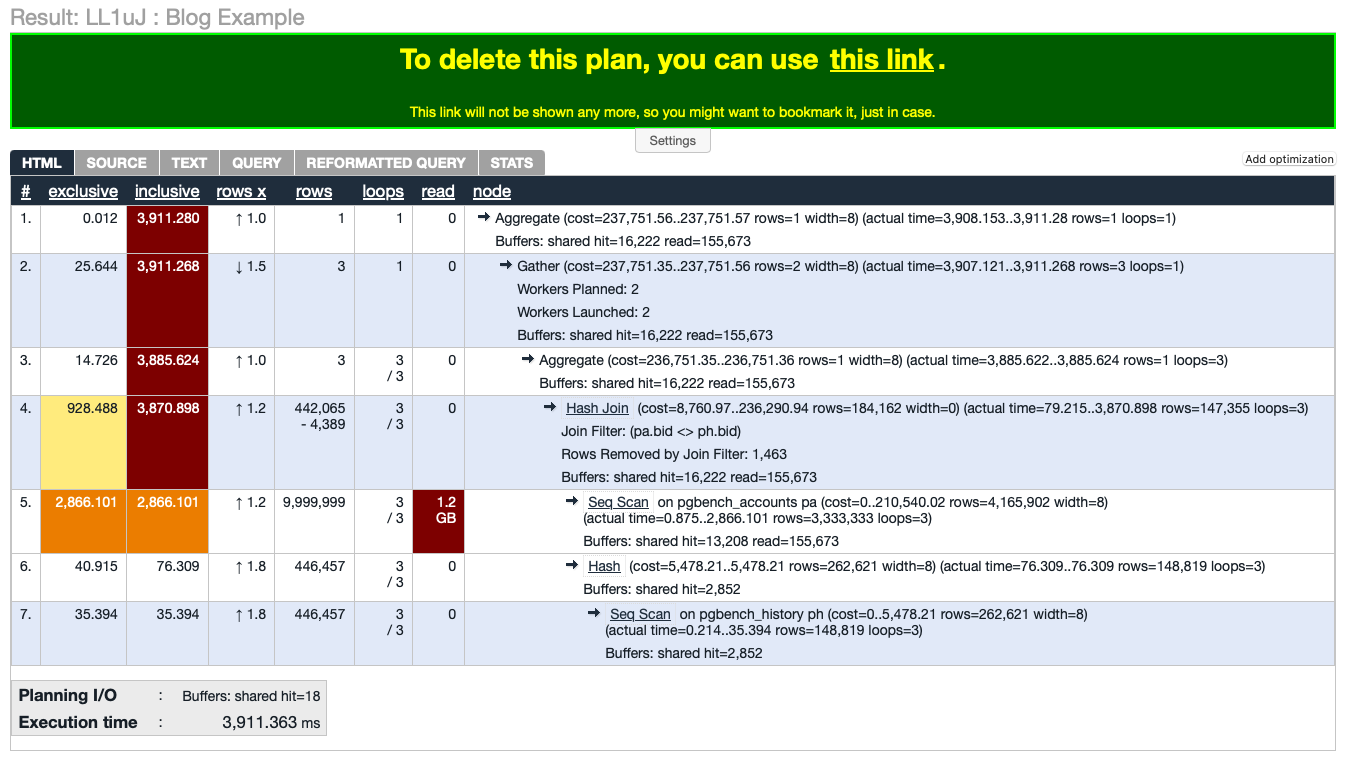 – Depesz
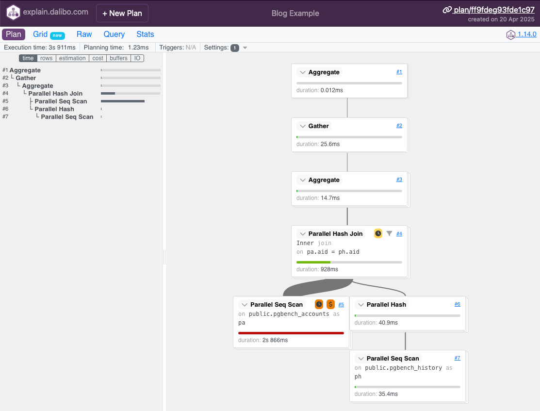 – Dalibo
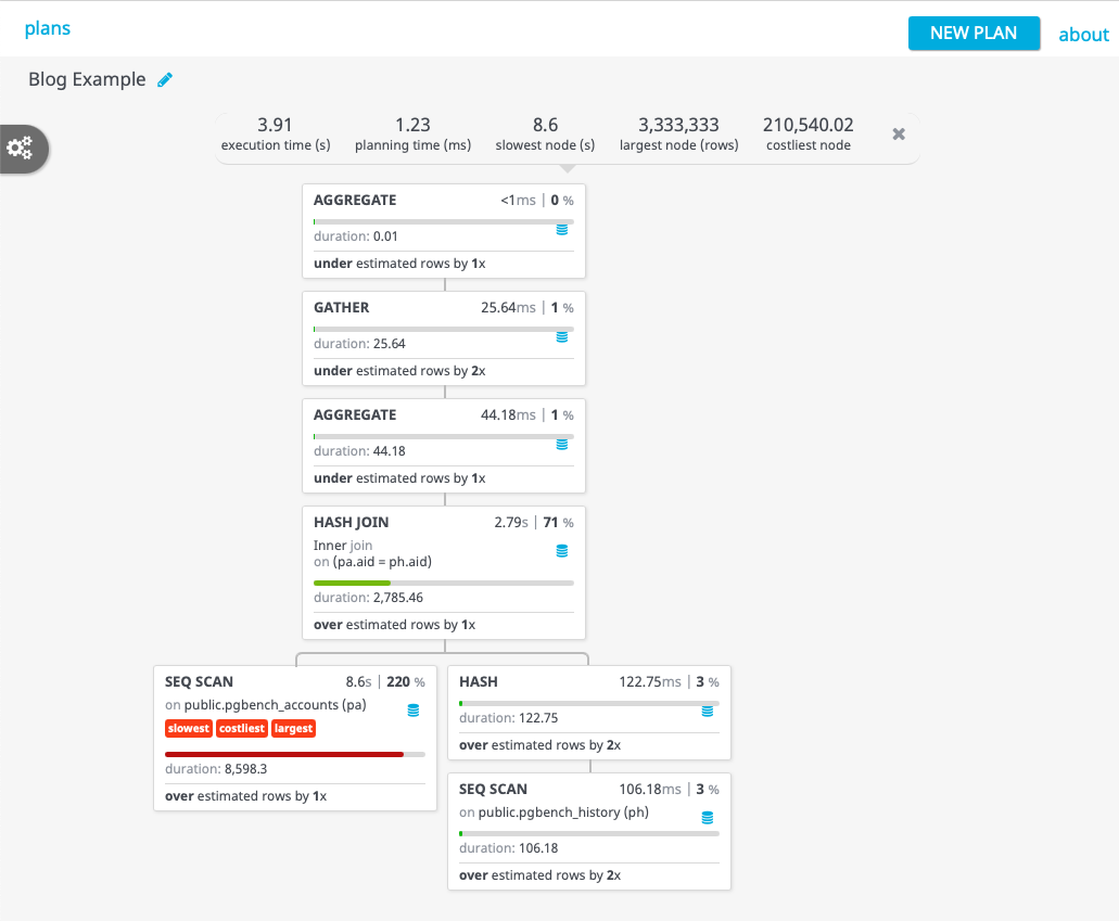 – PEV
– PEV
Red flags
One of the most obvious red flags in a query is a filter:
bench=# explain (costs, settings, verbose) select count(*) from pgbench_accounts pa join pgbench_history ph on pa.aid = ph.aid where pa.bid != ph.bid and pa.filler is not null;
Finalize Aggregate  (cost=237751.56..237751.57 rows=1 width=8)
  Output: count(*)
  ->  Gather  (cost=237751.35..237751.56 rows=2 width=8)
        Output: (PARTIAL count(*))
        Workers Planned: 2
        ->  Partial Aggregate  (cost=236751.35..236751.36 rows=1 width=8)
              Output: PARTIAL count(*)
              ->  Parallel Hash Join  (cost=8760.97..236290.94 rows=184162 width=0)
                    Hash Cond: (pa.aid = ph.aid)
                    Join Filter: (pa.bid <> ph.bid)  <<<=== This is a filter
                    ->  Parallel Seq Scan on public.pgbench_accounts pa  (cost=0.00..210540.02 rows=4165902 width=8)
                          Output: pa.aid, pa.bid, pa.abalance, pa.filler
                          Filter: (pa.filler IS NOT NULL)  <<<=== This is a filter
                    ->  Parallel Hash  (cost=5478.21..5478.21 rows=262621 width=8)
                          Output: ph.aid, ph.bid
                          ->  Parallel Seq Scan on public.pgbench_history ph  (cost=0.00..5478.21 rows=262621 width=8)
                                Output: ph.aid, ph.bid
Time: 2.402 ms
A filter is a strong indicator of a missing index, especially if a nested loop join is chosen by the optimiser..
Another red flag is a “large” number returned as the cost for a query. Large in this case is a slightly nebulous term, but a “fast” query will generally have a cost of tens of thousands or less.
Also look out for a large number of Rows Removed by Index Recheck or Rows Removed by Filter.
Costs vs durations
It’s important to note that there is not a consistent, reliable relationship between query cost and duration. I’ve had queries that returned costs over a million that ran faster than my example query above that returns costs of around 275,000. In general though, all you can say is that if two queries return the same result set, the one with the lower cost should be the fastest.
You cannot say that the cost is half, so it will take half the time. I’ve had queries where the starting costs were over ten million, after tuning the costs dropped to just over one million, but the duration dropped from minutes to sub-second.
Data considerations
Data distribution
if your data is not evenly distributed, then data distribution can lead to intermittent performance issues. For example, if you most of your customers are corner shops, but you also have Walmart/ASDA as a customer, then it’s quite likely that processing ASDA invoices will be a lot slower than everyone else, just because there’s more data. But this could also stem from a query plan being chosen that is good for the average customer, but is not optimal for ASDA.
For example, in pgbench:
bench=# select bid, count(*) from pgbench_accounts group by bid order by bid;
 bid | count
-----+--------
   1 | 100000
   2 | 100000
   3 | 100000
   4 | 100000
   5 | 100000
   6 | 100000
   7 | 100000
   8 | 100000
   9 | 100000
  10 | 100000
.
.
.
  90 | 100000
  91 | 100000
  92 | 100000
  93 | 100000
  94 | 100000
  95 | 100000
  96 | 100000
  97 | 100000
  98 | 100000
  99 | 100000
 100 | 100000
(100 rows)

bench=# select bid, count(*) from pgbench_history group by bid order by bid;
 bid | count
-----+-------
   1 |  4425
   2 |  4525
   3 |  4403
   4 |  4329
   5 |  4403
   6 |  4375
   7 |  4474
   8 |  4376
   9 |  4606
  10 |  4537
.
.
.
  90 |  4479
  91 |  4607
  92 |  4586
  93 |  4440
  94 |  4437
  95 |  4518
  96 |  4388
  97 |  4601
  98 |  4619
  99 |  4384
 100 |  4366
(100 rows)
As you can see, pgbench_accounts is perfectly evenly distributed across bids, and while pgbench_history is less evenly distributed, nothing stands our as wildly out of range.
Test data vs real data
Another thing to watch out for is trying to identify issues or fix issues based on test data. Test data rarely looks like production data, so apart from quality issues, there are also likely to be different data distributions from production.
Query optimisation
Projection
The first step in query optimisation is to ensure that you’re only returning the columns that you need. Networking is still one of the slowest parts of getting input from users and output to users. This is especially true in the always-online world of 3G and 4G.
Warning: SELECT *
Never use SELECT * in your application code. Even if you need every column, list them explicitly. The reason for this is that the table structure might change, but you might not have updated your code to reflect this change. This is highly likely to cause your application to crash.
Selection
The next optimisation is to limit the number of rows returned. Always return as few rows as possible. For example, don’t return thousands of transactions to a mobile application, return the data in page sized chunks. Chances are that the user will not make much sense of thousands of transactions anyway!
Linking data across tables
Joins are one of the most difficult things for an optimiser to assess correctly. The first thing to note is that optimisation complexity increases exponentially with each additional table. Therefore, join as few tables as possible. After five tables, most bets are off.
The next thing to be aware of is that there are multiple ways of linking tables, which are discussed below. Sometimes, the optimiser will return the exact same plan for two different ways, but it is unlikely that all approaches will return the same plan.
SQL-92
select count(*)
from pgbench_accounts pa
	join pgbench_history ph on pa.aid = ph.aid
where pa.bid != ph.bid
and pa.filler is not null;

Finalize Aggregate  (cost=237751.56..237751.57 rows=1 width=8)
  Output: count(*)
  ->  Gather  (cost=237751.35..237751.56 rows=2 width=8)
        Output: (PARTIAL count(*))
        Workers Planned: 2
        ->  Partial Aggregate  (cost=236751.35..236751.36 rows=1 width=8)
              Output: PARTIAL count(*)
              ->  Parallel Hash Join  (cost=8760.97..236290.94 rows=184162 width=0)
                    Hash Cond: (pa.aid = ph.aid)
                    Join Filter: (pa.bid <> ph.bid)
                    ->  Parallel Seq Scan on public.pgbench_accounts pa  (cost=0.00..210540.02 rows=4165902 width=8)
                          Output: pa.aid, pa.bid, pa.abalance, pa.filler
                          Filter: (pa.filler IS NOT NULL)
                    ->  Parallel Hash  (cost=5478.21..5478.21 rows=262621 width=8)
                          Output: ph.aid, ph.bid
                          ->  Parallel Seq Scan on public.pgbench_history ph  (cost=0.00..5478.21 rows=262621 width=8)
                                Output: ph.aid, ph.bid
Subquery
select count(*)
from pgbench_accounts pa
where pa.aid in (
	select ph.aid
	from pgbench_history ph
	where pa.bid != ph.bid
)
and pa.filler is not null;

Aggregate  (cost=47679947805.51..47679947805.52 rows=1 width=8)
  Output: count(*)
  ->  Seq Scan on public.pgbench_accounts pa  (cost=0.00..47679935307.81 rows=4999083 width=0)
        Output: pa.aid, pa.bid, pa.abalance, pa.filler
        Filter: ((pa.filler IS NOT NULL) AND (SubPlan 1))
        SubPlan 1
          ->  Seq Scan on public.pgbench_history ph  (cost=0.00..8432.70 rows=441991 width=4)
                Output: ph.aid
                Filter: (pa.bid <> ph.bid)
SQL-89
select count(*)
from pgbench_accounts pa, pgbench_history ph
where pa.aid = ph.aid
and pa.bid != ph.bid
and pa.filler is not null;

Finalize Aggregate  (cost=237751.56..237751.57 rows=1 width=8)
  Output: count(*)
  ->  Gather  (cost=237751.35..237751.56 rows=2 width=8)
        Output: (PARTIAL count(*))
        Workers Planned: 2
        ->  Partial Aggregate  (cost=236751.35..236751.36 rows=1 width=8)
              Output: PARTIAL count(*)
              ->  Parallel Hash Join  (cost=8760.97..236290.94 rows=184162 width=0)
                    Hash Cond: (pa.aid = ph.aid)
                    Join Filter: (pa.bid <> ph.bid)
                    ->  Parallel Seq Scan on public.pgbench_accounts pa  (cost=0.00..210540.02 rows=4165902 width=8)
                          Output: pa.aid, pa.bid, pa.abalance, pa.filler
                          Filter: (pa.filler IS NOT NULL)
                    ->  Parallel Hash  (cost=5478.21..5478.21 rows=262621 width=8)
                          Output: ph.aid, ph.bid
                          ->  Parallel Seq Scan on public.pgbench_history ph  (cost=0.00..5478.21 rows=262621 width=8)
                                Output: ph.aid, ph.bid
As you can see, SQL-89 and SQL-92 return the exact same query plan, but the subquery plan produces a query plan with a much higher cost. And rightly so, because the query has been running for nearly 48 hours now and is still not finished!
^CCancel request sent
ERROR:  canceling statement due to user request
Time: 160784555.953 ms (1 d 20:39:44.556)
Summary
In this post we looked at:
- Identifying slow queries by logging
- Using EXPLAIN to examine a query plan
- REMEMBER: EXPLAIN (ANALYZE) executes the query, beware!
- Visualizing query plans
- Red flags in the explain plan
- Data considerations
- The basics of query optimisation
Previous: Bloat and TOAST | Next: Indexing